What is YOLO ?
YOLO (You Only Look Once) networks are a very popular family of deep convolutional networks for real-time object detection. Real-time object detection models need to output predictions very fast, usually under 200 ms or process video streams at 30 FPS or more. In order to meet the speed requirements they are often smaller than non real-time models which often reduces precision.
The first yolo version was proposed in May 2016 by Joseph Redmon. He explained his novel idea with the paper “You Only Look Once : Unified Real-Time Object Detection”. As the name suggests, the main novelty of YOLO is that you only need to process an image once, a trait that provides great speedup during object detection.
The YOLO architecture became a great success in computer vision and 8 more versions followed after that ! The latest of which, YOLO-NAS, was released in may 2023, no longer after YOLOv8. Many deep learning practitioners use yolo object detection in their applications, with YOLOv8 probably being the most popular and widely used due to its great open source repository that offers an easy and abstract implementation.
What makes YOLO different ?
The main advantage of YOLO is its unparalleled inference speed. Previous object detection architectures would use an image classifier. In contrast YOLO’s novelty is that it changed the paradigm from classification to regression. Older architectures repurposed image classifiers and used them for object detection. Architectures like deformable parts models (DPM) use the sliding window technique, scanning subregions of an image with a moving window and applying a classifier on each subregion searching for the object of interest. On the other hand, R-CNN used the region proposal method that first generated proposal bounding boxes upon which the classifier would do the classification. The region proposal method offered a more noble method compared to the “brute force” technique of sliding window, but still multiple classifications need to be executed and post-processing is needed to eliminate duplicate detections. Such pipelines are slow and difficult to optimize.
YOLO changed the paradigm by transforming the object detection problem from classification to regression. Bounding box coordinates and class probabilities are being regressed directly from image pixels. You only need to look and classify an image once. A single convolutional neural network predicts multiple bounding boxes. Advantages :
- Fast : It’s able to achieve real-time object detection, >40 FPS.
- Simple : It only relies on a single convolutional neural network which outputs both the bounding box coordinates but also the class probabilities. R-CNN, in comparison, consists of 3 different modules[3].
- Trains on whole images : Since it trains on whole images it learns more generalized features. It sees both object and context (background). Hence, it is less prone to false positives due to background pixels.
How original YOLO object detector operates
Before we describe the different YOLO versions up to YOLO-NAS, it’s wise to explain the inference operation of the original YOLO model. The steps below are also visually presented in figure 1.
- The input image is separated into an SxS grid, where S in an adjustable hyperparameter. Each grid cell is responsible for detecting objects whose centers fall into that grid cell.
- Each grid cell predicts B bounding boxes, where B is again an adjustable hyperparameter. For every box it also outputs a confidence score (0.0 to 1.0) which represents how confident the model is that an object exists in the box and how accurate the box is. Essentially confidence is just the IOU(ground truth, prediction) , but formally it’s calculated as
P(object) * IOU(ground truth, prediction)
to account for the cases where no object exists in the box, since the probability will be zero.
- For each box Bi the model outputs 5 regression predictions (x, y, w, h, confidence). Variables x,y determine the object’s bounding box center while w, h are the box’s width and height.
- The model also outputs a “classification” prediction for each grid cell, which represents the probability of the class Classi being present inside a grid cell.
- The final score is calculated as shown below and it encodes both the accuracy of the bounding box and the class-specific classification confidence **.
Score = P(Classi| obj)* P(obj) *IOU = P(Classi)*IOU
All in all, the model will output an S S (B*5 + len(Class)) tensor, meaning that for each cell we have 5 outputs per bounding box (related to its position and fitness) and len(Class) outputs, one for each class in the dataset.
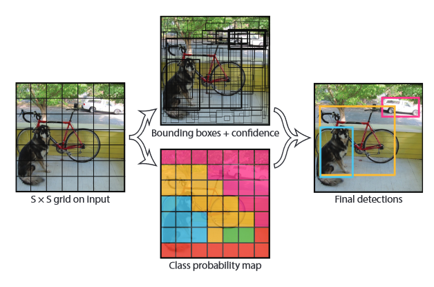
- **Note : A limitation for YOLO is that it can only predict one class per grid cell.
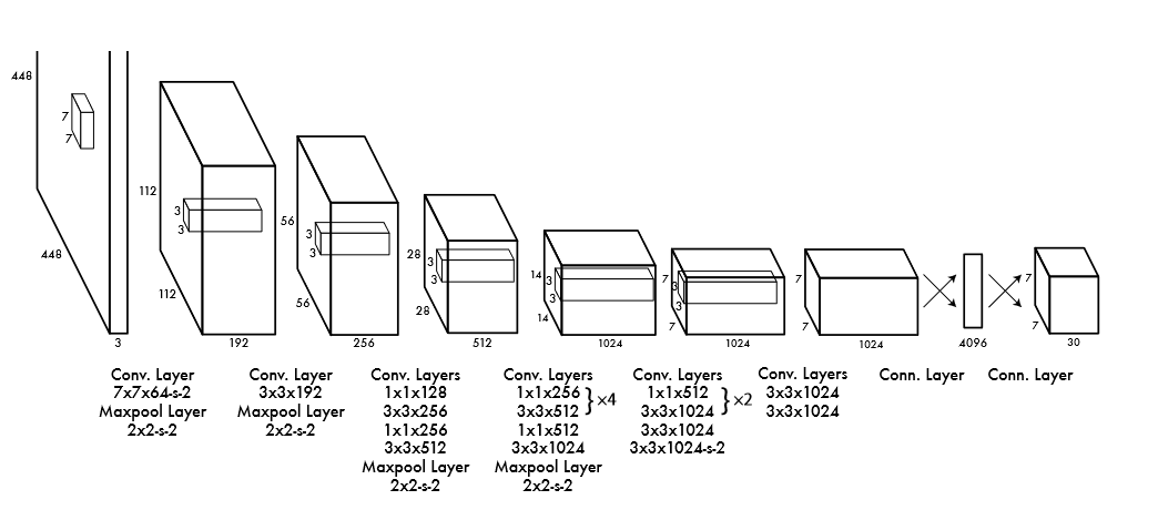
The image below presents the original YOLO architecture, which consists of a single CNN !
The architecture follows the typical paradigm of reducing image and kernel dimensions while increasing the number of filters in each conv layer along the way. A fully connected layer is also used in the end.
A history of YOLOs ( yolo9000, yolov3, yolov4, yolov5, yolov6, yolov7, yolov8, yolo nas)
Now that we understand the original yolo object detection model, let’s examine the subsequent versions.
YOLO 9000 (Yolov2)
YOLO 9000’s name derives from the capacity of the model to predict 9000 different classes. It builds upon the original architecture adding some features and discarding others, to increase performance. Joseph Redmon is again the main author and contributor to this model.
The most notable improvements are
- Includes Batch Normalization. The regularizing effects improved mAP by 2% .
- The pre-trained on ImageNet classifier used in YOLO accepts images of 224x224 but increases resolution to 448x448 during detection. To help the network adjust to different sizes, the classification network is first trained for 10 epochs on 448x448 images. This provided a 4% increase in mAP !
- Fully connected layers, on the prediction layer, are replaced with a Convolutional layer with Anchor boxes. Anchor boxes are pre-defined bounding boxes that act as suggestions for the network when it makes predictions. Essentially, when using anchors, the network only needs to correct the suggestions rather than discover it all by itself. Using anchors, mAP dropped by a slight 0.3%, however recall increased by a surprising 7% !
- Good anchor box priors were discovered by clustering the bounding box coordinates of the training set, instead of hand picking them.
- Applied a multiscale training technique, where the network gets trained on various resolutions to create more general representations.
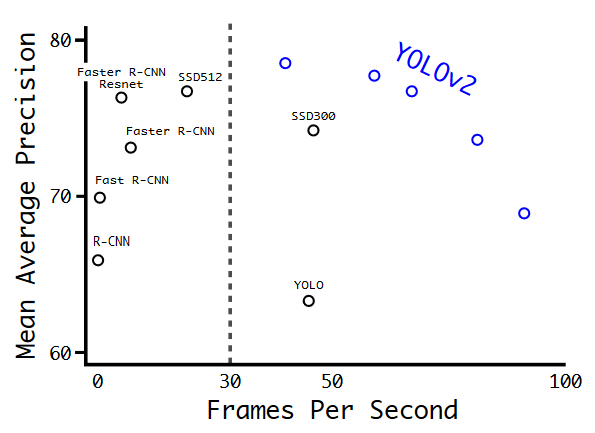
Fig 3 : Yolo 9000 became state-of-the-art. It was faster and more accurate than its competitors. Image Source [2]
YOLOv3 :
Yolov3, the last model by Joseph Redmon, was presented in a paper with a very humorous and sarcastic tone ! It is worth a read just for that. The model itself is slightly better and even though it didn’t rank with its competitors as good as YOLOv2 in terms of mAP, its inference speed is 3x times faster than its fastest competitor, an SSD variant. Achieves AP=33.0%
Multiple different CNN backbones were chosen, with DarkNet-19 being extremely fast reaching up to 171 FPS ! Residual connections, a golden standard nowadays, were also introduced in this version.
YOLOv4 :
The first model from the YOLO family, that doesn’t stem from University of Washington and Joseph Redmon but is still built on the DarkNet framework. The model was evaluated on the COCO dataset and provided surprising improvements in terms of AP while still being significantly faster than its competitors. Achieves AP=43.0%
Yolov4 mainly focused on improving its training methods. They used what they call “Bag of Freebies”, i.e. methods that only affect training and improve performance. Examples include
- Advanced augmentation methods (CutMix, Mosaic augmentation, Self-Adversarial Training)
- Replacing MSE loss with an IoU Loss variance
- Using DropBlock regularization and
- Finding the most optimal hyperparameters through genetic algorithms.
However, they also used “Bag of Specials”, i.e. plug-in blocks or post-processing methods that slightly increase inference cost but significantly improve the accuracy of object detections. Examples include
- Using mish activation function [6]
- Using Multi-input Weighted Residual Connections (MiWRC)
- Spatial Pyramid Pooling [7]
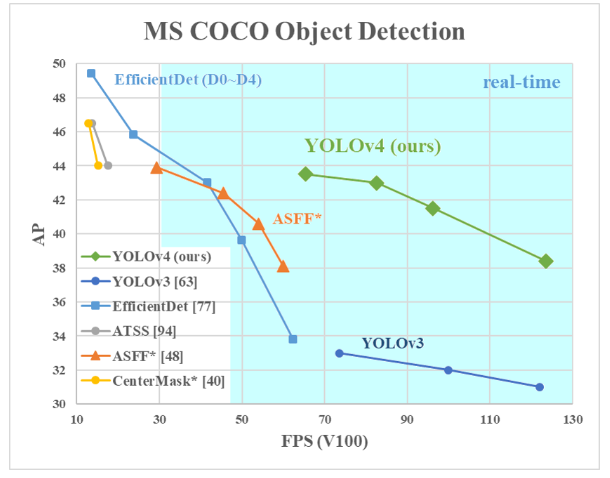
Fig 4 : Performance comparison of YOLOv4, YOLOv3 and competitor networks in COCO object detection dataset. Image Source [5]
YOLOv5 :
Shortly after the release of YOLOv4 Glenn Jocher from Ultralytics introduced YOLOv5 using the Pytorch framework, in May 2020. Due to this open source yolov5 repo [8], yolov5 is probably the most popular version of them all but also the most controversial.
No paper accompanied this version. The major difference from yolov4 is that yolov5 is built from source with the Pytorch library instead of being forked from the original DarkNet yolo.
A lot of controversy surrounds the versioning from yolov5 and onwards (v6, v7), with some claiming that they are unofficial. What really matters, though, is that people find these repositories useful and can build useful applications on top of their open source code.
YOLOv6 :
Yolov6 was released almost in parallel with Yolov7 (summer 2022), from the Chinese company Meituan. The aim was to test recent computer vision state of the art training methods and plug-in blocks. Explaining all of these intricate techniques is not the aim of this blog post but we briefly mention the main contributions of Yolov6.
- New RepVGG backbone model
- TAL : Task Alignment Learning
- VariFocal classification loss and SIoU/GIoU regression loss.
- Self-Distillation
- Quantization - Aware Training, for improved performance via weight quantization.
According to the benchmarks published in their paper, Yolov6 achieves up to AP=52.5% at 98 FPS with their largest model.
YOLOv7 :
YOLOv7, whose paper was published earlier than yolov6 paper (The versioning is getting messy…), managed to push the barriers of real-time object detection even further. According to their published paper “ YOLOv7 surpasses all known object detectors in both speed and accuracy in the range from 5 FPS to 160 FPS and has the highest accuracy 56.8% AP among all known real-time object detectors with 30 FPS or higher on GPU V100 “.
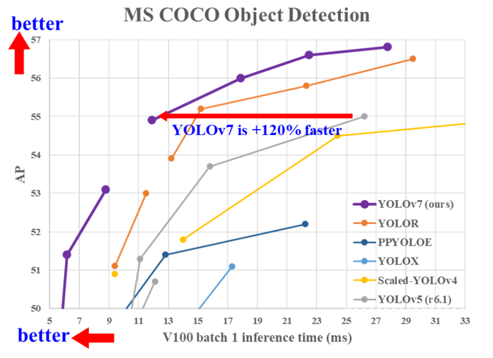
Fig. 5 : Comparison of yolov7 to other competitors. Yolov7 is currently SOTA in real time object detection. Image Source [10]
So effectively, YOLOv7 is the state of the art real time object detector for 2022. The paper is named “YOLOv7: Trainable bag-of-freebies sets new state-of-the-art for real-time object detectors”. So similarly to Yolov4 (same main author), they employ a number of state-of-the-art training methods for computer vision during training. This allows them to improve performance on COCO dataset without affecting inference speed at all. Everything they did only affects the computational training costs without compromising inference speed.
YOLOv8 :
Yolov8’s or the “Real-Time Flying Object Detection” was released in 2023. This new version is built as a unified framework for training models on different tasks such as detection, segmentation, pose estimation, tracking, and classification.
It uses a more advanced backbone network, which is a variant of the CPSDarkNetBackbone architecture. It uses both Feature Pyramid Network (FPN) and Path Aggregation Network (PAN), and it introduced improvements and new features to enhance performance as we can see on the following figures.
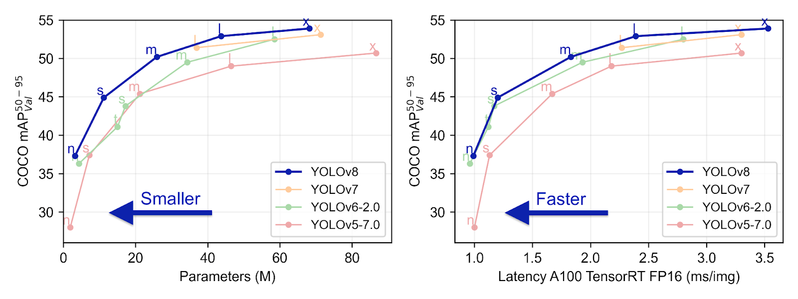
Faster, and more accurate than YOLOv7 and all their predecessors thanks to its multi-scale prediction, YOLOv8 constitute a powerful deep learning for real-time object detection. Its anchor free architecture also make it easier to use.
YOLOv8 also runs on CPUs and GPUs, and is highly efficient and flexible, supporting a wide range of export formats.
YOLO-NAS
According to DeciAI, YOLO-NAS is around 0.5 mAP points more accurate and 10% to 20% faster than equivalent variants of YOLOv8 and YOLOv7.
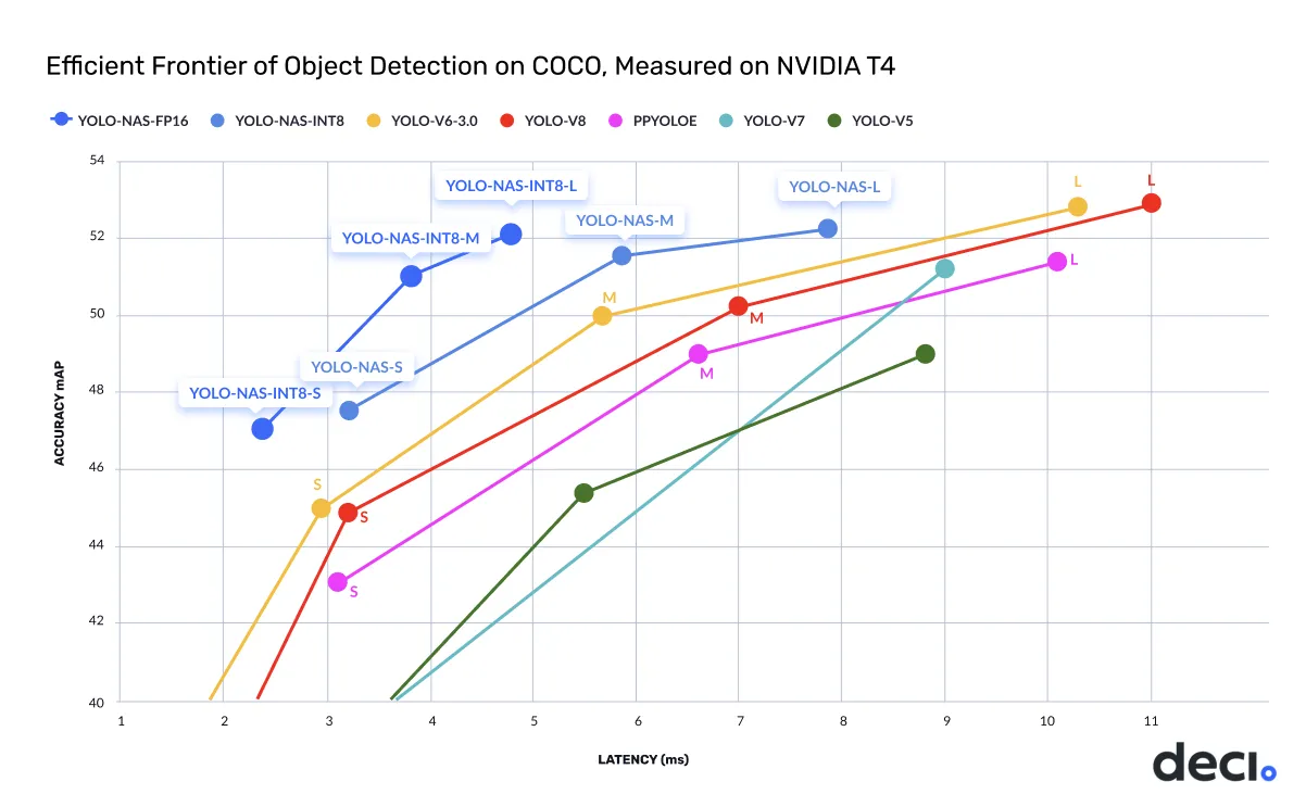
This version, developed by DeciAI aims to address the limitations of the previous models version in object detection. NAS, meaning Neural Architecture Search, is a technique for automating the design of artificial neural networks.
The three key features of YOLO-NAS highlight by Deci.ai are:
- Quantization-Friendly Basic Block
- Advanced Training and Quantization : advanced training schemes and post training quantization
- AutoNAC Optimization and Pre-training : make it perfectly suitable for real-world object detection
The model, when converted to its INT8 quantized version, experiences a minimal precision drop, a significant improvement over other models. These advancements culminate in a superior architecture with unprecedented object detection capabilities and outstanding performance.
Open source code for YOLO
Yolo object detectors are an excellent choice for real-time applications. If fast predictions are a requirement then YOLOv8 is probably the best choice at the moment. All yolo versions have open source codebases.
Working with them should be easy but you need to make sure your datasets’ annotations are in the yolo format.
Yolo bounding box annotations :
come in .txt format and every image should be accompanied by a .txt annotation file. Each row in the .txt file represents 1 object. In each row 5 identifiers are included that refer to the [class id, bbox center x, bbox center y , bbox width, bbox height] as presented in figure 6 below. It’s important to note that Class ID begins from number 0 and that coordinates are normalized in the [0,1] range. If your boxes are in pixels, divide center_x and bbox_width by image width, and center_y and bbox_height by image height.
You can annotate your datasets and export them in various formats using simple tools like LabelMe or use Picselia’s AI-assisted labeling tools and significantly decrease annotation costs.

Fig 6 : Example of yolo annotation file
Github Repositories :
- YOLOv5 is the most popular and well documented project with many official tutorials. Working with it is relatively easy and performance is usually good. However, it’s not state-of-the-art anymore.
- Yolov6 is also well documented and should provide better performance and speed compared to yolov5. If you are interested in training a yolov6 model with custom data this tutorial should prove useful. For a simple application all it takes is a few lines of code in the terminal after cloning their repo.
- Yolov7 repository offers more than just object detection. It’s easy to use their pre-trained model for pose estimation and instance segmentation. However, they do not provide as good documentation as yolov6/yolov5 and training on your custom data may require a bit more effort from your side. If you want to test the model, they also serve their model on the Hugging Face Spaces.
- yolov8 · GitHub Topics
- YOLONAS.md - Deci-AI/super-gradients
Conclusions
The YOLO model family has been a great success and that is reflected by the number of different versions that followed the original publication. Deep learning practitioners use yolo models for object detection since they provide an excellent trade-off between speed and accuracy. Working with yolo models is easy thanks to the open source repositories that have been published by the creators. Object detection is the main task that yolos are successful at, but yolov8 repository also serves models for classification, image segmentation and pose estimation.


