The Fastest Way to Analyze Models for Object Detection
Learn how to choose, tune and train any deep learning architecture to train your object detection models, by using an MLOps solution for computer vision.
Picsellia Team
·8 min read

Ready to build computer vision?
Go from raw images to production models. Free trial, no credit card, cancel anytime.
Today, training an object detection model should be an easy task, but some can still struggle. In this article, we will learn how to choose, tune and train any deep learning architecture seamlessly to counter this problem.
Do you ever feel that you can’t keep up with all the new trendy models that come out of labs every days?
To me, it seems like I see plots like this everyday.
 model benchmark.jfif
As I used to train Yolov3 a few years ago and it was awesome, I thought it'd be a great idea to check those brand new architectures and create even better models!
So I started searching for tutorials, Github repos, or even pre-trained weights so I could start using these new fancy architectures on my own data to see if I could produce better AI models for my company’s tasks.
But the truth is, even if I found the resources to train these architectures, I usually ended up feeling like the results were not far greater than those I managed to get a few years ago.
Is it my fault? Did I make any mistake in my code? Maybe my dataset isn’t that good? How can I rapidly know if it’s better than other models?
How can you really be sure of your ability to train and reproduce results? How can you make sure to always have the best architecture at the tips of your fingers? And how can you finally choose the best algorithms for your business problems?
That’s what we will cover in this article. We'll divide this piece in the following parts:
- Choose a suited dataset for object detection
- Select a bunch of models and create training scenarios
- Compare the training logs and metrics
- Compare the performances live on some images
Let’s get right into it!
**For the sake of simplicity, we will use Picsellia platform as it gives us a great panel of tools to do all the above tasks seamlessly. **To learn more about Picsellia's features, click here.
Choose a Dataset
As we are going to train models for an object detection task we have to choose a dataset for… you get it! Object Detection!
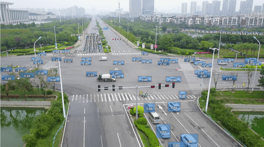
In order to obtain significant results, we will train our models on ~6500 images annotated with 144,000 cars and 106,000 pedestrians, and it looks like this.
 ground truth example.png
The dataset is called VizDrone and can be found fully annotated with 11 different classes on Picsellia.
Select models
Picsellia offers some ready-to-use SOTA architectures, including the most recent ones (for example EfficientDet-dx).
 some available architectures.png
For our test, we will compare the following architectures (brand new ones against older ones):
- efficientDet-d0 (base efficientDet)
- efficientDet-d2 (heavier efficientDet)
- faster-rcnn-resnet50 (older model)
- ssd-mobilenet-640 (lighter older model)
First, let’s create a project where we can schedule training for each of this model.
 project dashboard.png
Next, Create Your Experiments
Once Our dataset is well attached, we need to create different experiments.
We will create some ‘dummy’ experiments, meaning that we'll not try to optimize the hyperparameters in this article (don’t worry, we will cover this subject on a different parameter).
That said, I will keep the default parameters proposed by Picsellia and use the very same parameters for each and every experiment so we only have to compare the architectures.
Create a training scenario.
 experiment setup panel.png
We'll initialize our different tests with this dedicated UI where we can select a base model from the ones we saw earlier and have already configured optimal parameters.
After repeating the operation for all models we can check that we have everything set up.
 list of experiment.png
Looks good! If we go to any of the experiment and check the files, we can see that we have successfully cloned all the needed files for training from the pre-trained models.
 experiment files.png
Now, we just have to launch training and save every metric and log to the platform, made possible by Picsellia’s Python SDK.
One way to do it is to check the ‘launch’ tab in one of the experiments and copy the command to launch the pre-packaged Docker image ready for training.
(For obvious reasons we have blurred our account and project token but you can replace those with your own)
 docker snippet for training.png
Now, I will just copy & paste this command in our server equipped with NVIDIA GPUs and see the magic happen!
Let’s do this with the 4 experiments we just created and then wait a few hours for the training of the whole thing.
Compare The Results
If your trainings are all over, you can now go back to Picsellia, and in your experiment list, select them all and then click on ‘Compare’.
Now you should see a dashboard of all the different training logs, evaluation metrics, etc.
 the experiment dashboard.png
What can we conclude from our trained models?
To perform a first, really simplistic analysis, we will only look at a few evaluation metrics:
- the mAP (mean Average Precision)
- the AR (Average Recall)
And some of the training logs :
- the Total-Loss
If you're not familiar with those metrics and want to learn about them in detail I encourage you to check this blog post that explains everything in depth.
 learning rate for all exps.png
Here, we can see that our models are learning something as the loss curve is slowly decreasing. But it’s quite noisy…
To solve that, as we have a lot of training images we could try to increase the batch size during training, set the learning rate to decay faster than it actually does (see next figure) or use other more advanced techniques.
What we can learn from this plot is that the **efficientDets **model seems to converge faster than the other and that the variance of faster-rcnn doesn’t seem to decrease with time.
What you have to understand is that our analysis is in NO WAY exhaustive and that each architecture would need different parameters to optimize the training process. But this gives us a good intuition on how they behave comparing to each other, in a very little time.
 Learning rate for all experiments.png
If we sort our experiments based on the AR@10 score (the higher the better), we can see that our Faster-RCNN model seems to perform better than the other architecture. It means that this model will be the one that will most likely NOT make false predictions.
 metrics table (part 1).png
As I said, this is not a complete analysis and your job as a data scientist is to explore the models in depth so you can compare them once you have found the best parameters for each one.
Now that we have performed a little "quantitative" analysis, we will try our model on some images to see how they perform on real data.
Compare The Performances
In Picsellia you can find what is called a "Playground**"**. It's a place where you can try out models live right after you trained them and stored the weights and checkpoints.
For the test, we will use the following image where we can see the ground truth overlay. This image has been used for evaluation so it is not part of the training set.
 picsellia playground.png
Now we will try our models, adjust the threshold and see how they perform.
Here are the steps we observe in the animation above:
- Try efficientDet-d2 model and set a reasonable threshold
- Try all the other models with the same threshold
- Adjust the threshold until we can see some pedestrians
- Try all the models with this threshold
As we can see, it is** Faster-RCNN** the one that seems to perform best on our image, meaning that our previous little analysis wasn’t that far from truth!
 results with faster-rcnn.png
Conclusion
The goal of this article was to prove if we could rapidly identify, use and compare some model architectures (more or less new) and perform a quick analysis that would drive our future full exploratory experiments.
As we could observe, it’s not the newest, fancy architectures that perform the best with our first approach, which doesn’t mean that they can't increase in performance with a real, exhaustive training.
The whole thing took me half a day, training included, which is a good thing because that means that you don’t have to spend days or weeks (or even months) to explore your project and know for sure if it has a chance to succeed or not.
I hope that you enjoyed this article. If you think that **Picsellia **offers a very optimal way to run experiments and want to join, claim a trial here! We'll get back to you shortly, and get you started in no time.
See you soon! 👋
Related from Picsellia
Ship vision AI 10x faster
Picsellia is the end-to-end MLOps platform for computer vision — from data management to production deployment.
See the PlatformAutomate your ML pipelines
Set up continuous training and deployment with automated triggers, shadow deployments, and feedback loops.
Explore Automated PipelinesStay up to date
Get the latest posts on computer vision, MLOps, and AI delivered to your inbox.
Related articles

Picsellia at Big Data & AI Paris 2024
Read about Picsellia's experience at Big Data & AI Paris, 2024.

SAM and Foundation Models in Computer Vision
We explored how SAM was created to become such a powerful tool. A groundbreaking model not only for Meta, but for the entire computer vision scenario!

Is AutoML Replacing Data Scientists?
Machine Learning revolutionized computer vision and language processing and is now shapeshifting biology and engineering.